The homework requires Python 3.12. You do not need to install it yourself: the homework ships with a pyproject.toml pinned to 3.12, and uv sync (below) downloads that interpreter if it is missing. To confirm, run uv run python --version inside the homework directory after syncing.
Like previous assignments, we will use uv to set up the homework environment quickly.
Please refer to the official uv installation documentation for the most up-to-date installation instructions for your platform.
# Install uv once
curl -LsSf https://astral.sh/uv/install.sh | sh

# Optional: `uv` binary by default goes to `$HOME/.local/bin` on Linux/macOS,
# so you may need to add it to your PATH (uv may have done this for you):
export PATH="$HOME/.local/bin:$PATH"
# Install uv once
powershell -ExecutionPolicy ByPass -c "irm https://astral.sh/uv/install.ps1 | iex"
# Then open a NEW terminal window so that `uv` is on your PATH
# Download the homework zip and unzip into `hw6_bayesian/`
# In your hw directory (it ships with a pyproject.toml pinned to Python 3.12)
uv sync                   # Create .venv, fetch Python 3.12 if needed, install numpy, matplotlib, and einops
uv run python grader.py   # Run the local grader
If you prefer typing python directly, activate the environment first with source .venv/bin/activate (on Windows: .venv\Scripts\activate) and run commands with python instead, for example python grader.py and python submission.py 2d.
If you cannot run the assignment on your laptop or need additional computing resources, Stanford provides FarmShare, a community computing environment for coursework and unsponsored research. Please follow the instructions at https://docs.farmshare.stanford.edu/ to get started with the computing environment.
In this assignment, you will build Bayesian networks, sample from them to answer probabilistic queries (forward, rejection, and Gibbs sampling), and learn their parameters from data, first with every variable observed (maximum likelihood) and then with hidden variables (the EM algorithm).
You will only modify submission.py. Before you start coding, read the docstring at the top of util.py, which explains how Bayesian networks, conditional probability tables, and assignments are represented.
We've created a LaTeX template here for you to use that contains the prompts for each question. If you use Overleaf, also upload the plots you make in Problems 3 and 4 to include them.
What to Submitsubmission.py, submitted to the programming assignment on Gradescope. Upload the file itself, not a zip or folder, and check that the autograder results appear after a few minutes. If the autograder crashes, you will receive a 0 on the programming part.As in lecture, we write random variables with capitalized names (like $\text{Rain}$ or $Y$) and their values in lowercase (like $r$ or $y$), and we always say which value a variable takes. For example, $\mathbb{P}(\text{Rain} = 1)$ is a number, the probability that it rained, and $\mathbb{P}(\text{Rain} = r, \text{WetGrass} = w)$ is the probability that $\text{Rain}$ takes the value $r$ and $\text{WetGrass}$ takes the value $w$. We write $\mathbb{P}$ for probabilities under the joint distribution and $p$ for the local conditional distributions of a Bayesian network, often with the shorthand $p(r) = p(\text{Rain} = r)$ and $p(w \mid r, s) = p(\text{WetGrass} = w \mid \text{Rain} = r, \text{Sprinkler} = s)$.
Let's consider a simple scenario which we can model using a Bayesian network. You are walking to CS221 lecture and, on the way, you notice the grass on the Stanford Oval is wet. You reason that this could be because either it rained (rare in beautiful and sunny Palo Alto), or the sprinklers were on. Letting your mind wander from the lecture, you decide to sit down and figure out what happened here by applying your knowledge of Bayesian networks.
We use three binary variables: $\text{Rain} = 1$ if it rained and $\text{Rain} = 0$ if it did not, $\text{Sprinkler} = 1$ if the sprinklers were on and $0$ if they were off, and $\text{WetGrass} = 1$ if the grass is wet and $0$ if it is dry. Assume that the sprinklers run independently of the weather: whether they were on does not depend on whether it rained.
| $r$ | $s$ | $p(\text{WetGrass} = 1 \mid \text{Rain} = r, \text{Sprinkler} = s)$ |
| $1$ | $1$ | $0.9$ |
| $1$ | $0$ | $0.8$ |
| $0$ | $1$ | $0.7$ |
| $0$ | $0$ | $0.0$ |
You got distracted while examining that luscious green grass in the Stanford Oval, and you somehow wandered into the Gilbert Biological Sciences Building. As you realize where you are, you overhear some biologists discussing the genome of a new species they've discovered, provisionally given the scientific name Kenius bayus.
(As you remember from high school biology, the genome of a living thing is encoded in DNA, which is a long chain of nucleotides. Each nucleotide can be one of four organic molecules: A, C, T, or G.)
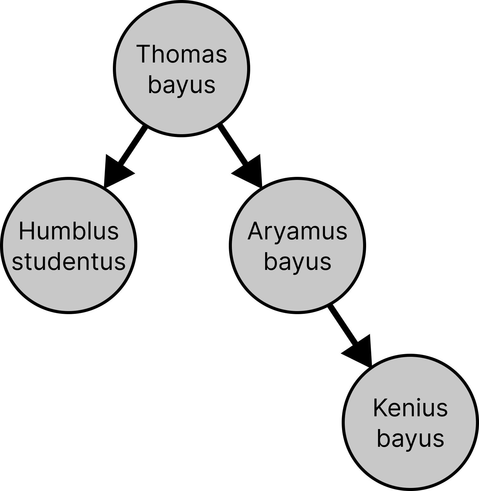
The figure shows how Kenius bayus is related to its ancestor, Thomas bayus, and two other species. We abbreviate the species as TB (Thomas bayus), HS (Humblus studentus), AB (Aryamus bayus), and KB (Kenius bayus).
The Bayesian network. A genome of length $L$ is a sequence of nucleotides at positions $j = 0, 1, \dots, L - 1$. Our Bayesian network has one variable per species per position: $\text{TB}_j \in \{\text{A}, \text{C}, \text{T}, \text{G}\}$ is the nucleotide of Thomas bayus at position $j$, and $\text{HS}_j$, $\text{AB}_j$, and $\text{KB}_j$ are the nucleotides of the other species at position $j$. At every position, the edges follow the tree in the figure: $\text{TB}_j \rightarrow \text{HS}_j$, $\text{TB}_j \rightarrow \text{AB}_j$, and $\text{AB}_j \rightarrow \text{KB}_j$. There are no edges between different positions.
Assume a simplified model of biology in which the nucleotides of Thomas bayus are uniformly distributed, and each descendant copies the nucleotide of its ancestor at each position, except that with probability mutation_rate it mutates to one of the other three nucleotides, chosen uniformly. Mutations at different positions are independent, and every position has the same local conditional distributions. For example, if we set mutation_rate = 0.1, then the local conditional distribution $p(\text{HS}_j = h \mid \text{TB}_j = t)$ is the following, for every position $j$:
| $t$ | $p(\text{HS}_j = \text{A} \mid \text{TB}_j = t)$ | $p(\text{HS}_j = \text{C} \mid \text{TB}_j = t)$ | $p(\text{HS}_j = \text{T} \mid \text{TB}_j = t)$ | $p(\text{HS}_j = \text{G} \mid \text{TB}_j = t)$ |
| $\text{A}$ | $0.9$ | $0.03333$ | $0.03333$ | $0.03333$ |
| $\text{C}$ | $0.03333$ | $0.9$ | $0.03333$ | $0.03333$ |
| $\text{T}$ | $0.03333$ | $0.03333$ | $0.9$ | $0.03333$ |
| $\text{G}$ | $0.03333$ | $0.03333$ | $0.03333$ | $0.9$ |
The same table gives $p(\text{AB}_j = a \mid \text{TB}_j = t)$ and $p(\text{KB}_j = k \mid \text{AB}_j = a)$, and $p(\text{TB}_j = t) = 1/4$ for every $t$. So the joint probability of four genomes is $$\mathbb{P}(\text{TB} = t, \text{HS} = h, \text{AB} = a, \text{KB} = k) = \prod_{j=0}^{L-1} p(t_j)\, p(h_j \mid t_j)\, p(a_j \mid t_j)\, p(k_j \mid a_j),$$ where $\text{TB} = t$ is short for $\text{TB}_0 = t_0, \dots, \text{TB}_{L-1} = t_{L-1}$. For example, with $L = 4$, $\text{TB} = \text{AAAC}$ means that $\text{TB}_0 = \text{TB}_1 = \text{TB}_2 = \text{A}$ and $\text{TB}_3 = \text{C}$.
In the code, a BayesianNode represents one species at all positions: its conditional probability table (CPT) is the local conditional distribution that all positions share. network.sequence_length is $L$, and an assignment maps each node's name to a list with one value per position: assignment['Thomas bayus'][j] is the value of $\text{TB}_j$.
The biologists are trying to figure out the probability of Kenius bayus's genome resulting from a series of mutations from its ancestor, Thomas bayus. You realize you could help these poor biologists, who never took CS221, by modeling the mutation process with Bayesian networks!
initialize_phylogenetic_tree, which converts the phylogenetic tree into a Bayesian network using the BayesianNetwork and BayesianNode classes defined in util.py.
An implementation of the initialize_phylogenetic_tree function in submission.py, which takes a mutation_rate and a genome_length and returns a BayesianNetwork with one node per species, with the CPTs given by the mutation model.
We provide the code that creates the BayesianNetwork with sequence_length = genome_length; you only need to define each node, with its domain, parents, and CPT.
Understanding the shape of the conditional probability table (CPT): The CPT of a BayesianNode is a numpy array with one axis per parent, in the order of node.parents, and a last axis for the node's own domain: cpt[i, ..., v] is the probability that the node takes the value node.domain[v] when its parents take the values with indices i, ... in their domains. For example, a node with two parents whose domains have length 4 and a domain of length 4 needs a CPT of shape (4, 4, 4), and a node without parents with a domain of length 4 has a CPT of shape (4,): its prior. All positions share the same CPTs, so the shapes don't depend on genome_length.
By default, the BayesianNode constructor creates uniform distributions over the domain, but for some problems you will need to set the CPTs to different distributions.
For later problems: Remember to read and understand the member functions of the BayesianNode class in util.py, particularly get_probability, parent_assignment_indices, and iter_parent_assignments, as well as the helper function values_at_position.
forward_sampling, which draws a single sample from the joint distribution of the given Bayesian network: one value for every variable at every position.
forward_sampling function in submission.py. At each position, go through the nodes in the order network.order (which puts parents before their children) and sample each node from its local conditional distribution given the values of its parents at that position, which you have already sampled. Your code should work for any Bayesian network and any network.sequence_length.
compute_joint_probability, which computes the joint probability of a full assignment to all the variables of a Bayesian network, at all positions.
compute_joint_probability function in submission.py: the product, over all positions and all nodes, of the local conditional probabilities. Your code should work for any Bayesian network and any network.sequence_length.
test_forward_sampling, which creates the network with mutation_rate = 0.1 and genome_length = 10 and then runs your forward_sampling function once on this network.
Run it with uv run python submission.py 2d, and fill out the table below with the complete genomes you observed for each species.
| Species | Genome |
| Thomas bayus | |
| Humblus studentus | |
| Aryamus bayus | |
| Kenius bayus |
rejection_sampling, which takes a network, the name of the target variable, the evidence (a partial assignment, such as {'Kenius bayus': ['A', 'A', 'A', 'A']}), and the number of samples to draw, and returns the estimated distribution of the target variable given the evidence.
rejection_sampling function in submission.py, which should call the forward_sampling function you implemented in part (b). It returns a dictionary that maps each value of the target variable that appears in a kept sample, as a tuple with one value per position (e.g. ('A', 'A', 'A', 'C')), to its estimated probability, or an empty dictionary if no sample agrees with the evidence.
gibbs_sampling function, which takes the same arguments as rejection_sampling, except that it takes the number of iterations instead of the number of samples. We have implemented the initialization for you: the state starts as a sample from forward_sampling, with the evidence variables set to the evidence. Each iteration should resample every non-evidence variable at every position from its distribution given all the other variables in the state, and then record the value of the target variable.
You may assume that every entry of every CPT is strictly positive (for the phylogenetic tree, this holds whenever mutation_rate is strictly between 0 and 1), so the joint probabilities you normalize never all equal zero.
gibbs_sampling function in submission.py. Its return value has the same format as the return value of rejection_sampling.
Hint: the probability that a variable takes the value $v$ given all the other variables is proportional to the joint probability of the state with that variable set to $v$, since the other factors of the joint probability don't depend on $v$. So you can use your compute_joint_probability.
rejection_sampling and gibbs_sampling, estimate $\mathbb{P}(\text{TB} = \text{AAAC} \mid \text{KB} = \text{AAAA})$ with the provided benchmarking function test_gibbs_vs_rejection, which you can run with uv run python submission.py 2g (a step is a sample for rejection sampling and an iteration for Gibbs sampling). Fill out the table below with the results.
With only 100 steps, rejection sampling usually keeps no samples, because the evidence $\text{KB} = \text{AAAA}$ is rare, so it will often print an estimate of $0.0000$. That is expected and not a bug: record the estimate that it prints.
| Method | Steps/Iterations | Estimated Posterior |
| Rejection sampling | 100 | |
| Rejection sampling | 10,000 | |
| Gibbs sampling | 100 | |
| Gibbs sampling | 10,000 | |
| Exact | — |
Later in life, you're a data engineer managing a team of human annotators. Your data consists of labels indicating whether a given conversation between an LLM and a human was good or bad.
But you've run into a problem: your annotators can't seem to perfectly agree on their ratings, no matter how careful you are in your instructions! You vaguely remember something about Bayesian networks from CS221, so you decide to use them to help you assess annotator quality.
For this problem, we'll assume you have the true labels for each conversation. (In the real world, this will not be the case!) Also assume that each annotator's label depends only on the true label of the conversation, and that annotators make mistakes independently of each other: once you know the true label, how one annotator labeled the conversation tells you nothing about how another one did.
| $y$ | $p(A_0 = \text{good} \mid Y = y)$ | $p(A_0 = \text{bad} \mid Y = y)$ |
| $\text{good}$ | ||
| $\text{bad}$ |
| $y$ | $p(A_0 = \text{good} \mid Y = y)$ | $p(A_0 = \text{bad} \mid Y = y)$ |
| $\text{good}$ | ||
| $\text{bad}$ |
bayesian_network_for_annotators(num_annotators), which returns the Bayesian network for one conversation that you will use for the rest of this assignment. It has a node Y for the true label, with a uniform prior, and one node per annotator (A_0, A_1, A_2, ...; 0-indexed), with Y as its only parent. All nodes have the domain ['good', 'bad'].
bayesian_network_for_annotators function in submission.py. EM in Problem 4 starts from the annotator CPTs you choose here, so they should encode a reasonable prior that annotators are better than chance but not perfect: for each annotator $A_k$ and each label $y$, $p(A_k = y \mid Y = y)$ should be greater than $0.5$ and less than $1$.
Datasets. Each example in a dataset is one conversation: an assignment such as {'Y': ['good'], 'A_0': ['good'], 'A_1': ['bad'], 'A_2': ['good']}, where each list has one value because the annotator network has sequence_length = 1. The provided function load_annotation_csv returns a list of these examples, one per row of the dataset. All conversations share the same CPTs, so you learn the parameters by counting over all the examples.
lambda_param instead of 0.
Implement the helper function accumulate_assignment, which adds the (weighted) counts of one full assignment, and the function mle_estimate, which takes a BayesianNetwork, a list of fully observed examples, and lambda_param, and sets the CPTs of the network to their smoothed maximum likelihood estimates.
accumulate_assignment and mle_estimate functions in submission.py. You should use the provided helper functions init_zero_conditional_probability_tables (which creates count tables of zeros with the shapes of the CPTs) and normalize_counts (which turns count tables into CPTs) where applicable; you don't need to implement them.
data/annotations.csv with labels from 3 annotators for 100 conversations. Note that this dataset contains the true label of each conversation. Implement mle_estimate_for_annotators, which takes the list of labeled examples and returns the annotator network for 3 annotators, with its parameters learned by your mle_estimate (with the default lambda_param = 1).
mle_estimate_for_annotators function in submission.py.
uv run python submission.py 3g, which reads the dataset, learns the parameters with your mle_estimate_for_annotators, and plots the CPT of each annotator with plot_annotator_cpts (saved to plots/annotators.png). Which annotator seems to be the least trustworthy, and why?
Your real dataset doesn't actually have the true labels. You thus want to both model the annotator noise and estimate the true labels.
You must now use the Expectation Maximization (EM) algorithm from lecture. Starting from the initial CPTs of the network, EM repeats two steps:
Implement the algorithm and analyze the results on the dataset.
e_step(network, data), which returns the list of completions of all the examples in data (each a full assignment) and the list of their weights $q(h)$. (You should be able to use functions you implemented earlier as subroutines.)
e_step function in submission.py, which uses your compute_joint_probability. An example without hidden variables gives a single completion, the example itself, with weight 1.
Tip: you should normalize the weights for each example in the dataset independently, e.g. the weights of all the completions of the first example should sum to $1$.
m_step(network, completions, weights), which takes the completions and weights from the e_step function and sets the CPTs of the network to their maximum likelihood estimates on the weighted completions (without smoothing).
m_step function in submission.py. Your code should use your earlier implementation of accumulate_assignment and the provided init_zero_conditional_probability_tables and normalize_counts.
em_learn(network, data, num_iterations), which runs the EM algorithm for a given number of iterations, starting from the current CPTs of the network.
em_learn function in submission.py.
uv run python submission.py 4d, which calls the provided function test_em_learn to train the annotator network on the unlabeled dataset with 100 iterations of your em_learn, starting from the CPTs of your bayesian_network_for_annotators. It saves two plots:
plots/annotators_em.png: the learned CPT of each annotator, made with plot_annotator_cpts.plots/labels_em.png: made with plot_label_posteriors, histograms of the posterior $\mathbb{P}(Y = \text{good} \mid \text{annotations})$ of every conversation under the learned network, shown separately for the conversations whose true label is good and bad. (EM never sees the true labels; we only use them to make this plot.)submission.py |
Where you will write your code, and the only file you submit. |
util.py |
The BayesianNode and BayesianNetwork classes, helpers for counting, loading the dataset, and plotting. |
grader.py |
The local grader, with the basic tests and the inputs of the hidden tests. |
data/annotations.csv |
The annotation dataset for Problems 3 and 4: the true label and the label from each of 3 annotators for 100 conversations. |