This assignment is a modified version of the Driverless Car assignment written by Chris Piech.
A study by the World Health Organization found that road accidents kill a shocking 1.24 million people a year worldwide. In response, there has been great interest in developing autonomous driving technology that can drive with calculated precision and reduce this death toll. Building an autonomous driving system is an incredibly complex endeavor. In this assignment, you will focus on the sensing system, which allows us to track other cars based on noisy sensor readings.
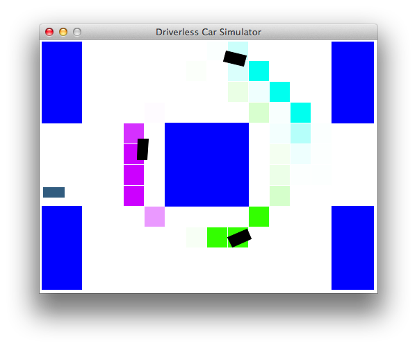
Getting started. You will be running two files in this assignment - grader.py and drive.py. The drive.py file is not used for any grading purposes, it's just there to visualize the code you will be writing and help you gain an appreciation for how different approaches result in different behaviors (and to have fun!). Let's start by trying to drive manually.
python drive.py -l lombard -i none
You can steer by either using the arrow keys or 'w', 'a', and 'd'. The up key and 'w' accelerates your car forward, the left key and 'a' turns the steering wheel to the left, and the right key and 'd' turns the steering wheel to the right. Note that you cannot reverse the car or turn in place. Quit by pressing 'q'. Your goal is to drive from the start to finish (the green box) without getting in an accident. How well can you do on the windy Lombard street without knowing the location of other cars? Don't worry if you're not very good; the teaching staff were only able to get to the finish line 4/10 times. An accident rate of 60% is pretty abysmal, which is why we're going to use AI to do this.
Flags for python drive.py:
-a: Enable autonomous driving (as opposed to manual).-i <inference method>: Use none, exactInference, particleFilter to (approximately) compute the belief distributions over the locations of the other cars.-l <map>: Use this map (e.g. small or lombard). Defaults to small.-d: Debug by showing all the cars on the map.-p: All other cars remain parked (so that they don't move).
At each time step $t$, let $C_t \in \mathbb R^2$
be a pair of coordinates representing the actual location of
the single other car (which is unobserved).
We assume there is a local conditional distribution $p(c_t \mid c_{t-1})$ which
governs the car's movement.
Let $a_t \in \mathbb R^2$ be your car's position,
which you observe and also control.
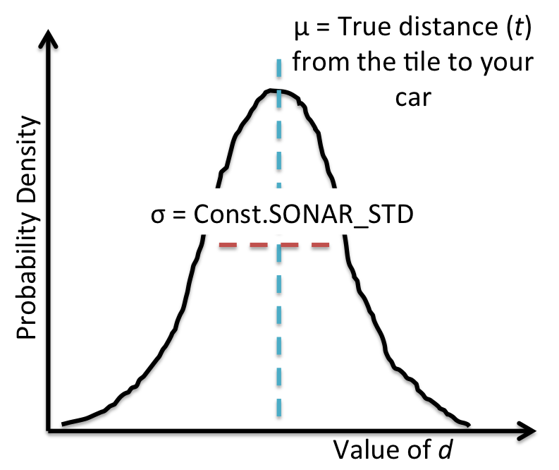
To minimize costs, we use a simple sensing system based on a microphone.
The microphone provides us with $D_t$,
which is a Gaussian random variable with mean equal
to the true distance between your car and the other car
and variance $\sigma^2$ (in the code, $\sigma$ is Const.SONAR_STD, which
is about two-thirds the length of a car).
In symbols,
For example, if your car is at $a_t = (1,3)$ and the other car is
at $C_t = (4,7)$, then the actual distance is $5$ and $D_t$ might be $4.6$ or $5.2$, etc.
Use util.pdf(mean, std, value) to compute the
probability density function (PDF)
of a Gaussian with given mean mean and standard deviation std, evaluated at value.
Note that evaluating a PDF at a certain value does not return a probability -- densities can exceed $1$ --
but for the purposes of this assignment, you can get away with treating it like
a probability.
The Gaussian probability density function for the noisy distance
observation $D_t$, which is centered around your distance to the car $\mu =
\|a_t - C_t\|$, is shown in the following figure:
Your job is to implement a car tracker that (approximately) computes the posterior distribution $\mathbb P(C_t \mid D_1 = d_1, \dots, D_t = d_t)$ (your beliefs of where the other car is) and update it for each $t = 1, 2, \dots$. We will take care of using this information to actually drive the car (i.e., set $a_t$ to avoid a collision with $c_t$), so you don't have to worry about that part.
To simplify things, we will discretize the world into tiles
represented by (row, col) pairs,
where 0 <= row < numRows
and 0 <= col < numCols.
For each tile, we store a probability representing our belief that there's a car on that tile.
The values can be accessed by:
self.belief.getProb(row, col).
To convert from a tile to a location,
use util.rowToY(row) and util.colToX(col).
Here's an overview of the assignment components:
ExactInference,
which computes a full probability distribution of another car's location over
tiles (row, col).ParticleFilter,
which works with particle-based representation of this same distribution.A few important notes before we get started:
First, let us look at a simplified version of the car tracking problem. For this problem only, let $C_t \in \{0, 1\}$ be the actual location of the car we wish to observe at time step $t \in \{1, 2, 3\}$. Let $D_t \in \{0, 1\}$ be a sensor reading for the location of that car measured at time $t$. Here's what the Bayesian network (it's an HMM, in fact) looks like:
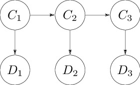
The distribution over the initial car distribution is uniform; that is, for each value $c_1 \in \{0, 1\}$: $$ p(c_1) = 0.5. $$ The following local conditional distribution governs the movement of the car (with probability $\epsilon$, the car moves). For each $t \in \{2, 3\}$: $$ p(c_t \mid c_{t-1}) = \begin{cases} \epsilon & \text{if $c_t \neq c_{t-1}$} \\ 1-\epsilon & \text{if $c_t = c_{t-1}$}. \end{cases} $$ The following local conditional distribution governs the noise in the sensor reading (with probability $\eta$, the sensor reports the wrong position). For each $t \in \{1, 2, 3\}$: $$ p(d_t \mid c_t) = \begin{cases} \eta & \text{if $d_t \neq c_t$} \\ 1-\eta & \text{if $d_t = c_t$}. \end{cases} $$
Below, you will be asked to find the posterior distribution for the car's position at the second time step ($C_2$) given different sensor readings.
Important: For the following computations, try to follow the general strategy described in lecture (marginalize non-ancestral variables, condition, and perform variable elimination). Try to delay normalization until the very end. You'll get more insight than trying to chug through lots of equations.
i. Compute and compare the probabilities $\mathbb P(C_2 = 1 \mid D_2 = 0)$ and $\mathbb P(C_2 = 1 \mid D_2 = 0, D_3 = 1)$. Give numbers, round your answer to 4 significant digits.
ii. How did adding the second sensor reading $D_3 = 1$ change the result? Explain your intuition for why this change makes sense in terms of the car positions and associated sensor observations.
iii. What would you have to set $\epsilon$ to be while keeping $\eta = 0.2$ so that $\mathbb P(C_2 = 1 \mid D_2 = 0) = \mathbb P(C_2 = 1 \mid D_2 = 0, D_3 = 1)$? Explain your intuition in terms of the car positions with respect to the observations.
In this problem, we assume that the other car is stationary (e.g., $C_t =
C_{t-1}$ for all time steps $t$).
You will implement a function observe that upon observing a new
distance measurement $D_t = d_t$ updates the current posterior probability from
$$\mathbb P(C_t \mid D_1 = d_1, \dots, D_{t-1} = d_{t-1})$$
to
$$\mathbb P(C_t \mid D_1 = d_1, \dots, D_t = d_t) \propto \mathbb P(C_t \mid D_1 = d_1, \dots, D_{t-1} = d_{t-1}) p(d_t \mid c_t),$$
where we have multiplied in the emission probabilities $p(d_t \mid c_t)$ described earlier under "Modeling car locations".
The current posterior probability is stored as self.belief in ExactInference.
observe method in
the ExactInference class of submission.py.
This method should modify self.belief in place to update the posterior
probability of each tile given the observed noisy distance to the other car.
After you're done, you should be able to find the stationary
car by driving around it (using the flag -p means cars don't move):Notes:
python drive.py -a -p -d -k 1 -i exactInferenceYou can also turn off
-a to drive manually.
drive.py on your local machine, but if you do decide
to run it on cardinal/rice instead, please ssh into the farmshare machines with either
the -X or -Y option in order to get the graphical interface; otherwise, you will
get some display error message. Note: do expect this graphical interface to be a bit slow...
drive.py is not used for grading, but is just there for you to visualize and
enjoy the game!Belief class before you get started...
you'll need to use this class for several of the code tasks in this assignment.Now, let's consider the case where the other car is moving
according to transition probabilities $p(c_{t+1} \mid c_t)$.
We have provided the transition probabilities for you in self.transProb.
Specifically,
self.transProb[(oldTile, newTile)] is the probability of the other car
being in newTile at time step $t+1$ given that it was in oldTile at time step $t$.
In this part, you will implement a function elapseTime that updates
the posterior probability about the location of the car at a current time $t$
$$\mathbb P(C_t = c_t \mid D_1 = d_1, \dots, D_t = d_t)$$
to the next time step $t+1$ conditioned on the same evidence, via the recurrence:
$$\mathbb P(C_{t+1} = c_{t+1} \mid D_1 = d_1, \dots, D_t = d_t) \propto \sum_{c_t} \mathbb P(C_t = c_t \mid D_1 = d_1, \dots, D_t = d_t) p(c_{t+1} \mid c_t).$$
Again, the posterior probability is stored as self.belief in ExactInference.
ExactInference by implementing the
elapseTime method.
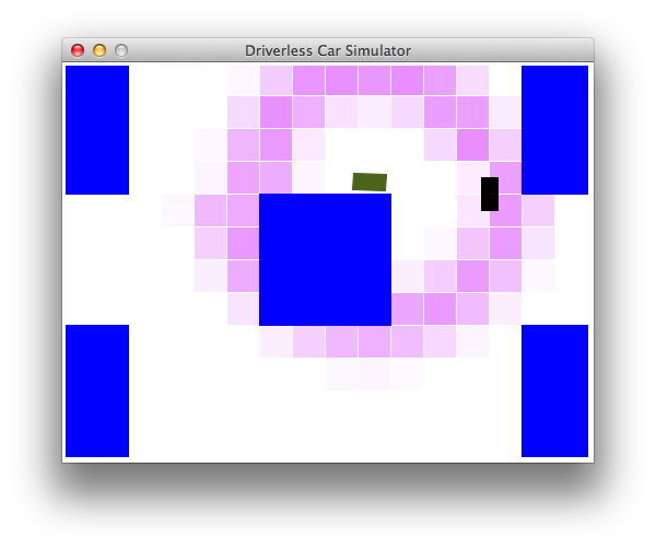
When you are all done, you should be able to
track a moving car well enough to drive autonomously by running the following.python drive.py -a -d -k 1 -i exactInference
Notes:
python drive.py -a -d -k 3 -i exactInference
python drive.py -a -d -k 3 -i exactInference -l lombardOn Lombard, the autonomous driver may attempt to drive up and down the street before heading towards the target area. Again, focus on the car tracking component, instead of the actual driving.
Though exact inference works well for the small maps, it wastes a lot of effort computing probabilities for every available tile, even for tiles that are unlikely to have a car on them. We can solve this problem using a particle filter. Updates to the particle filter have complexity that's linear in the number of particles, rather than linear in the number of tiles.
For a great conceptual explanation of how particle filtering works, check out this video on using particle filtering to estimate an airplane's altitude.
In this problem, you'll implement two short but important methods for the ParticleFilter
class in submission.py. When you're finished, your code should be able to track cars nearly
as effectively as it does with exact inference.
observe and elapseTime functions.
These should modify self.particles, which is a map from tiles (row, col) to the
number of particles existing at that tile, and self.belief, which needs to be updated each time
you re-sample the particle locations.
You should use the same transition probabilities as in exact inference. The belief distribution generated by a particle filter is expected to look noisier compared to the one obtained by exact inference.
python drive.py -a -i particleFilter -l lombardTo debug, you might want to start with the parked car flag (
-p) and the display car flag (-d).
Note: The random number generator inside util.weightedRandomChoice behaves differently
on different systems' versions of Python (e.g., Unix and Windows versions of Python).
Please test this question (run grader.py) on rice or Gradescope. When copying files to
rice, make sure you copy the entire folder using scp with the recursive option -r, i.e. scp -r car {your SUNet ID}@rice.stanford.edu:. You may need to install the python3.6+ in order to see the same behavior.
So far, we have assumed that we have a distinct noisy distance reading for each car, but in reality, our microphone would just pick up an undistinguished set of these signals, and we wouldn't know which distance reading corresponds to which car. First, let's extend the notation from before: let $C_{ti} \in \mathbb R^2$ be the location of the $i$-th car at the time step $t$, for $i = 1, \dots, K$ and $t = 1, \dots, T$. Recall that all the cars move independently according to the transition dynamics as before.
Let $D_{ti} \in \mathbb R$ be the noisy distance measurement of the $i$-th car at time step $t$, which is now not directly observed. Instead, we observe the set of distances $D_t = \{ D_{t1}, \dots, D_{tK} \}$. (For simplicity, we'll assume that all distances are distinct values.) Alternatively, you can think of $E_t = (E_{t1}, \dots, E_{tK})$ as a list which is a uniformly random permutation of the noisy distances $(D_{t1}, \dots, D_{tK})$. For example, suppose $K=2$ and $T = 2$. Before, we might have gotten distance readings of $1$ and $2$ for the first car and $3$ and $4$ for the second car at time steps $1$ and $2$, respectively. Now, our sensor readings would be permutations of $\{1, 3\}$ (at time step $1$) and $\{2, 4\}$ (at time step $2$). Thus, even if we knew the second car was distance $3$ away at time $t = 1$, we wouldn't know if it moved further away (to distance $4$) or closer (to distance $2$) at time $t = 2$.
Remember that $\mathcal p_{\mathcal N}(v; \mu, \sigma^2)$ is the probability of a random variable, $v$, in a Gaussian distribution with mean $\mu$ and standard deviation $\sigma$.
Hint: for $K=1$, the answer would be $$\mathbb P(C_{11} = c_{11} \mid E_1 = e_1) \propto p(c_{11}) p_{\mathcal N}(e_{11}; \|a_1 - c_{11}\|, \sigma^2).$$ where $a_t$ is the position of the car at time t. To better inform your use of Bayes' rule, you may find it useful to draw the Bayesian network and think about the distribution of $E_t$ given $D_{t1}, \dots, D_{tK}$.
You can also assume that the car locations that maximize the probability above are unique ($C_{1i} \neq c_{1j}$ for all $i \neq j$).
Note: you don't need to produce a complicated proof for this question. It is acceptable to provide a clear explanation based on your intuitive understanding of the scenario.