We've created a LaTeX template here for you to use that contains the prompts for each question.
Ensure that you're using Python version 3.12. Check your Python version by running:
python --version
or
python3 --version
.exe file to start the installation.chmod +x Miniconda3-latest-Linux-x86_64.sh
./Miniconda3-latest-Linux-x86_64.sh
.pkg file to start the installation.After installing Miniconda, set up your environment with the following commands:
conda create --name cs221 python=3.12
conda activate cs221
This homework does not require any additional packages, so feel free to reuse the cs221 environment you installed earlier for hw1 and hw2.
This assignment is a modified version of the Driverless Car assignment written by Chris Piech.
A study by the World Health Organization found that road accidents kill a shocking 1.24 million people a year worldwide. In response, there has been great interest in developing autonomous driving technology that can drive with calculated precision and reduce this death toll. Building an autonomous driving system is an incredibly complex endeavor. In this assignment, you will focus on the sensing system, which allows us to track other cars based on noisy sensor readings.
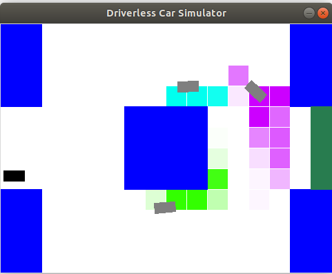
Getting started. You will be running two files in this assignment - grader.py and drive.py. The drive.py file is not used for any grading purposes, it's just there to visualize the code you will be writing and help you gain an appreciation for how different approaches result in different behaviors (and to have fun!). Let's start by trying to drive manually.
python drive.py -l lombard -i none
You can steer by either using the arrow keys or 'w', 'a', and 'd'. The up key and 'w' accelerates your car forward, the left key and 'a' turns the steering wheel to the left, and the right key and 'd' turns the steering wheel to the right. Note that you cannot reverse the car or turn in place. Quit by pressing 'q'. Your goal is to drive from the start to finish (the green box) without getting in an accident. How well can you do on the windy Lombard street without knowing the location of other cars? Don't worry if you're not very good; the teaching staff were only able to get to the finish line 4/10 times. An accident rate of 60% is pretty abysmal, which is why we're going to use AI to do this.
Flags for python drive.py:
-a: Enable autonomous driving (as opposed to manual).-i <inference method>: Use none, exactInference to compute the belief distributions over the locations of the other cars.-l <map>: Use this map (e.g. small or lombard). Defaults to small.-d: Debug by showing all the cars on the map.-p: All other cars remain parked (so that they don't move).Note: If any equations in the problems below aren't rendering properly (ex: you see a box outline where a symbol should presumably go), please either try using Safari or right click on the equation, then go Math Settings -> Math Renderer -> change it to anything other than HTML-CSS.
At each time step $t$, let $C_t \in \mathbb R^2$
be a pair of coordinates representing the actual location of
the single other car (which is unobserved).
We assume there is a local conditional distribution $p(c_t \mid c_{t-1})$ which
governs the car's movement.
Let $a_t \in \mathbb R^2$ be your car's position,
which you observe and also control.
To minimize costs, we use a simple sensing system based on a microphone.
The microphone provides us with $D_t$,
which is a Gaussian random variable with mean equal
to the true distance between your car and the other car
and variance $\sigma^2$ (in the code, $\sigma$ is Const.SONAR_STD, which
is about two-thirds the length of a car).
In symbols,
For example, if your car is at $a_t = (1,3)$ and the other car is
at $C_t = (4,7)$, then the actual distance is $5$ and $D_t$ might be $4.6$ or $5.2$, etc.
Use util.pdf(mean, std, value) to compute the
probability density function (PDF)
of a Gaussian with given mean mean and standard deviation std, evaluated at value.
Note that evaluating a PDF at a certain value does not return a probability -- densities can exceed $1$ --
but for the purposes of this assignment, your computations can get away with treating the returned PDF value like
a probability.
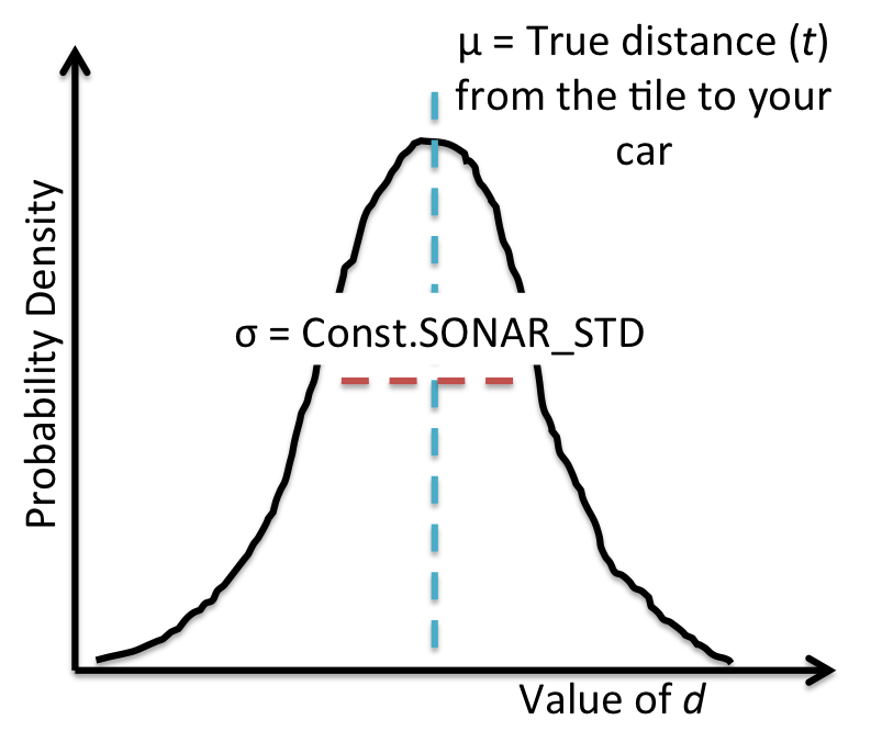
The Gaussian probability density function for the noisy distance
observation $D_t$, which is centered around your distance to the car $\mu =
\|a_t - C_t\|_2$, is shown in the following figure:
Your job is to implement a car tracker that (approximately) computes the posterior distribution $\mathbb P(C_t \mid D_1 = d_1, \dots, D_t = d_t)$ (your beliefs of where the other car is) and update it for each $t = 1, 2, \dots$. The helper code will take care of using this information to actually drive the car (i.e., set $a_t$ to avoid a collision with $c_t$), so you don't have to worry about that part.
To simplify things, we will discretize the world into tiles
represented by (row, col) pairs,
where 0 <= row < numRows
and 0 <= col < numCols.
For each tile, we store a probability representing our belief that there's a car on that tile.
The values can be accessed by:
self.belief.getProb(row, col).
To convert from a tile to a location,
use util.rowToY(row) and util.colToX(col).
Here's an overview of the assignment components:
ExactInference,
which computes a full probability distribution of another car's location over
tiles (row, col).A few important notes before we get started:
util.pdf instead of from util import * and referencing
pdf() directly. Also, don't use keyword arguments for util.pdf and just pass parameters
directly, e.g. util.pdf(mean, std, value) and not util.pdf(mean=mean, std=std, value=value)
In this problem, we assume that the single other car is stationary (e.g., $C_t =
C_{t-1} = C$ for all time steps $t$).
We'll denote the single variable representing the other car's stationary location as $C$,
and note that $p(C)$ is a known local conditional distribution.
You will implement a function observe that upon observing a new
distance measurement $D_t = d_t$ updates the current posterior probability from
$$\mathbb P(C \mid D_1 = d_1, \dots, D_{t-1} = d_{t-1})$$
to find the posterior for the next time step
$$\mathbb P(C \mid D_1 = d_1, \dots, D_t = d_t) $$
The current posterior probability is stored as self.belief in ExactInference.
observe method in
the ExactInference class of submission.py.
This method should modify self.belief in place to update the posterior
probability of each tile given the observed noisy distance to the other car.
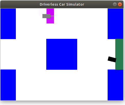
After you're done, you should be able to find the stationary
car by driving around it (using the flag -p means cars don't move):Notes:
python drive.py -a -p -d -k 1 -i exactInferenceYou can also turn off
-a to drive manually.
Belief class before you get started...
you'll need to use this class for several of the code tasks in this assignment.Now, let's consider the case where the other car is moving
according to transition probabilities $p(C_{t+1} \mid C_t)$.
We have provided the transition probabilities for you in self.transProb.
Specifically,
self.transProb[(oldTile, newTile)] is the probability of the other car
being in newTile at time step $t+1$ given that it was in oldTile at time step $t$.
Now, you will implement a function elapseTime that updates
the conditional probability about the location of the car at a current time $t$ $\mathbb P(C_t = c_t \mid D_1 = d_1, \dots, D_t = d_t)$
to the next time step $t+1$ conditioned on the same evidence, via the recurrence:
$$\mathbb P(C_{t+1} = c_{t+1} \mid D_1 = d_1, \dots, D_t = d_t) \propto \sum_{c_t} \mathbb P(C_t = c_t \mid D_1 = d_1, \dots, D_t = d_t) p(c_{t+1} \mid c_t).$$
Again, the posterior probability is stored as self.belief in ExactInference.
ExactInference by implementing the
elapseTime method.
When you are all done, you should be able to
track a moving car well enough to drive autonomously by running the following.python drive.py -a -d -k 1 -i exactInference
Notes:
python drive.py -a -d -k 3 -i exactInference
python drive.py -a -d -k 3 -i exactInference -l lombardOn Lombard, the autonomous driver may attempt to drive up and down the street before heading towards the target area. Again, focus on the car tracking component, instead of the actual driving.
So far, we have assumed that we have a distinct noisy distance reading for each car at each time step. In reality, our microphone would just pick up an undistinguished set of these signals, and we wouldn't know which distance reading corresponds to which car. We'll now consider this more realistic setting.
First, let's extend the notation from before: let $C_{ti} \in \mathbb R^2$ be the location of the $i$-th car at the time step $t$, for $i = 1, \dots, K$ and $t = 1, \dots, T$. Recall that all the cars move independently according to the transition dynamics as before.
Let $D_{ti} \in \mathbb R$ be the noisy distance measurement of the $i$-th car at time step $t$, which is no longer directly observed. Instead, we observe the unordered set of distances $\{ D_{t1}, \dots, D_{tK} \}$ as a collective and so cannot attribute any individual measurement in this set to a specific car. (For simplicity, we'll assume that all distances are distinct values.) In other words, you can think of this scenario as the same as observing the list $\mathbf{E_t} = [E_{t1}, \dots, E_{tK}]$ which is a uniformly random permutation of the (noisy) correctly ordered distances $\mathbf{D_t} = [D_{t1}, \dots, D_{tK}]$ where index $i$ represents the noisy distance to car $i$ at time $t$.
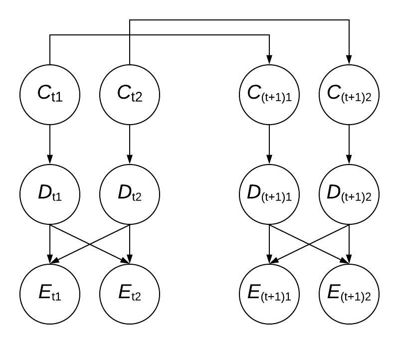
For example, suppose $K=2$ and $T = 2$. Before, we might have gotten distance readings of $8$ and $4$ for the first car and $5$ and $7$ for the second car at time steps $1$ and $2$, respectively. Now, our sensor readings would be permutations of $\{8, 5\}$ (at time step $1$) and $\{4, 7\}$ (at time step $2$). Thus, even if we knew the second car was distance $5$ away at time $t = 1$, we wouldn't know if it moved further away (to distance $7$) or closer (to distance $4$) at time $t = 2$.
Below is a diagram that shows the flow of information corresponding to the above situation for the case where $K = 2$ and only showing two timesteps, $t$ and $t+1$. Note that because the observed distances $\mathbf{E_t}$ are a permutation of the true distances $\mathbf{D_t}$, each $E_{ti}$ depends on all of the $D_{ti}$. Also note that the above diagram is not a Bayes net as $E_{t1}$ and $E_{t2}$ are not conditionally independent given $D_{t1}$ and $D_{t2}$ (however, $D_{t1}$ and $D_{t2}$ are conditionally independent given $C_{t1}$ and $C_{t2}$).
Remember that $\mathcal p_{\mathcal N}(v; \mu, \sigma^2)$ is the probability of a random variable, $v$, in a Gaussian distribution with mean $\mu$ and standard deviation $\sigma$.
Hint: for $K=1$, the answer would be $$p(C_{11} = c_{11} \mid \mathbf{E_1} = \mathbf{e_1}) \propto p(c_{11}) p_{\mathcal N}(e_{11}; \|a_1 - c_{11}\|_2, \sigma^2).$$ where $a_t$ is the position of your car (that you are controlling) at time $t$. Remember that $C_{ti}$ is the position of the $i$th observed car at time $t$. To better inform your use of Bayes' rule, you may find it useful to draw the Bayesian network and think about the distribution of $\mathbf{E_t}$ given $D_{t1}, \dots, D_{tK}$.
Hint: Note that the observed variable(s) are the shuffled/randomized distances $\mathbf{E_t} = [E_{t1}, E_{t2}, ..., E_{tK}]$. These are a random permutation of the unobserved noisy distances $\mathbf{D_t} = [D_{t1}, D_{t2}, ..., D_{tK}]$, where $D_{t1}$ is the distance of car $1$ at timestep $t$. Note that $E_{t1}$ is the emission from one of the cars at timestep $t$, but we aren't sure which one (it is NOT necessarily car 1, it could be any of the cars). On the other hand, $D_{t1}$ is the measured distance of car 1 (we know with certainty that it comes from car 1), the only issue is that we don't observe it directly.
Hint: To reduce notation, you may write, for example, $p(c_{11}∣e_{11})$ instead of $p(C_{11}=c_{11}∣E_{11}=e_{11})$.
You can also assume that the car locations that maximize the probability above are unique ($c_{1i} \neq c_{1j}$ for all $i \neq j$).
Hint: The priors $p(c_{1i})$ are a probability distribution over the possible starting positions ($t=1$) of each car $i$. Note that even if the car positions share the same prior, it doesn't necessarily mean they have the exact same start positions $c_{1i}$ because the start positions are sampled from the prior distribution, which can yield different values each time it is sampled from. However, you should think about what the priors all being the same means intuitively in terms of how we can associate observations with cars.
Note: you don't need to produce a complicated proof for this question. It is acceptable to provide a clear explanation based on your intuitive understanding of the scenario.
For reference, the treewidth of a factor graph is defined as the maximum arity (number of variables that a factor depends on) of any factor created by variable elimination under the best variable elimination ordering. You can find further information, along with an example, that may be relevant to this problem here.
Note: the conditioning is already done, so the only factors remaining are for $C_{ti}$ variables.Define auxiliary variables $z_1, z_2, \dots z_t$ which can be used to model the relation between $\mathbf{c_t}$ and $\mathbf{e_t}$. Give an expression for $p(\mathbf{c_t} \mid \mathbf{c_{t-1}})$ in terms of $\mathbf{e_1}, \cdots, \mathbf{e_t}$ and $z_t$.
submission.py ExactInferenceWithSensorDeception.observe() (we are using a technique called Box-Muller transform but you don’t need to know the details of this method for this problem). The skewness factor is set in the __init__ constructor with a default value of 0.5 (and you can assume the factor will always be greater than 0). Implement this change in the code and rerun python drive.py -a -p -d -k 3 -i exactInferenceWithSensorDeception to observe any changes.
submission.py observe() for class ExactInferenceWithSensorDeception.
python drive.py -a -d -k 3 -i particleFilter to observe the behavior. Comment on how the simulation looks different from the exact inference case and provide a reason why.
[2] See https://mit-serc.pubpub.org/pub/wrestling-with-killer-robots/release/2 and https://www.forbes.com/sites/cognitiveworld/2019/01/07/the-dual-use-dilemma-of-artificial-intelligence.
Submission is done on Gradescope.
Written: When submitting the written parts, make sure to select all the pages
that contain part of your answer for that problem, or else you will not get credit.
To double check after submission, you can click on each problem link on the right side, and it should show
the pages that are selected for that problem.
Programming: After you submit, the autograder will take a few minutes to run. Check back after
it runs to make sure that your submission succeeded. If your autograder crashes, you will receive a 0 on the
programming part of the assignment. Note: the only file to be submitted to Gradescope is submission.py.
More details can be found in the Submission section on the course website.